MachineX: Understanding FP-Tree construction

Table of contents

Reading Time: 5 minutes

In my previous blog, MachineX: Why no one uses apriori algorithm for association rule learning?, we discussed one of the first algorithms in association rule learning, apriori algorithm. Although even after being so simple and clear, it has some weaknesses as discussed in the above-mentioned blog. A significant improvement over the apriori algorithm is FP-Growth algorithm.

To understand how FP-Growth algorithm helps in finding frequent items, we first have to understand the data structure used by it to do so, the FP-Tree, which will be our focus in this blog.

FP-Tree

To put it simply, an FP-Tree is a compressed representation of the input data. It is constructed by reading the dataset one transaction at a time and mapping each transaction onto a path in the FP-Tree structure. As different transactions can have same items, their paths may overlap.

Above figure is an example of an FP-Tree. It consists of a root node which is represented by null. Then the given dataset in the figure is iterated transaction by transaction and the nodes corresponding to different items are made in the FP-Tree. The nodes contain the item they are representing and a counter which tells how many times that item has repeated in this path, thus avoiding its storage multiple times and providing compression. The FP-Tree made in first three iterations is shown in the figure with the final FP-Tree. As you can see in the figure, two different branches are made for first two transactions, as their prefix was not common. You can see a dotted line from b from the first transaction to the b from the second transaction. This line represents that both the nodes are linked through a linked list. This makes their retrieval very fast. When mapping the third transaction on the FP-Tree, a was common for TID 1 and 3, so a‘s counter was increased and from it, another branch was created to represent TID 3. Following a similar approach, the final FP-Tree was constructed after reading all 10 transactions.

Let’s dive into the construction of FP-Tree to clearly understand what FP-Tree is.

FP-Tree Construction

We will see how to construct an FP-Tree using an example. Let’s suppose a dataset exists such as the one below –

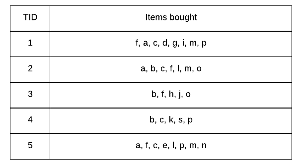
For this example, we will be taking minimum support as 3.

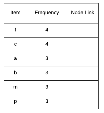
Step 1 – List down the frequencies of the individual items in the dataset.

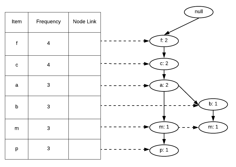
Step 2 – Eliminate frequencies lower than minimum support and arrange the remaining frequencies in descending order. Add another column to this table with the name ‘Node Link’. This column consists of the pointer pointing to the linked list containing nodes with same items. For example, in the description of FP-Tree, while reading TID 2, we made a new branch for that transaction and b in both the transactions were linked as they were part of a linked list. This table is known as the Header Table.

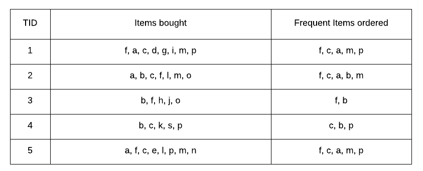
Step 3 – Order items in every transaction in frequency descending order, and items with support lesser than minimum support eliminated.

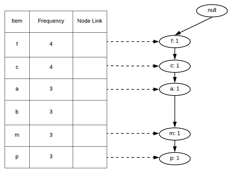
Step 4 – We will use Frequent Items ordered column to build our FP-Tree. We will iterate it transaction by transaction. We will initialize our FP-Tree with a root node represented by null. Then we will pick the first transaction, in this case, {f, c, a, m, p}, and since no node exists in the FP-Tree, make a branch from the root node and assign it the item f and initialize its counter to 1, since we have only encountered it 1 time till now. We will also link the header table to the newly created node f. Then we will look at the next item in the transaction which is c. We will create a branch from node f and create another node and assign it the item c with the counter as 1 and link the header table to this node. Below figure shows the FP-Tree created after the first transaction has been fully traversed.

Step 5 – After the first transaction has been fully traversed, we will move onto our next transaction in the dataset, which is {f, c, a, b, m}. We notice here that f, c and a have already occurred before as can also be seen in the FP-Tree created till now. So, instead of creating a new branch for them, we will just increment their counters, and from a we will create a new branch for b and m. Notice that even if an item has already occurred before but is now occurring with a different prefix, we will have to create a new branch for it, that is what we are doing here for m. After traversing the second transaction, we will have the FP-Tree as shown in the below figure.

We can see that we have already achieved some level of compression here by mapping f, c and a on the same branch.

Step 6 – We will repeat this process for all the transactions in the dataset. Finally, after traversing the whole dataset, we will get an FP-Tree and header table as shown in the below figure.

Overlapping is what provides us with the blessing of compression here. Due to overlapping, a repeated item in different itemsets is stored in just one node of the tree while it is repeated in the actual data. So as you can already guess, the worst case of an FP-Tree would be when there is no overlapping, i.e., all the items in the dataset are unique and non-repeating, which is a very rare case and hardly ever occurs. In that scenario, FP-Tree would consist of the same number of nodes as the items in the actual data, although FP-Tree would require a little more memory to store the pointers and the counters of each node, so actually in worst case scenario, its space complexity would be worse than the actual space complexity of the input data. But again, that case hardly ever happens, so FP-Tree can be used almost every time.

Now that we have constructed the FP-Tree, we will have to extract the frequent patterns from it, where we will make use of the FP-Growth algorithm, which we will pick up in our next blog. Till then, stay tuned!

References –