

This is my third blog post on MR-REX, a software package used to help determine protein structures given experimental X-ray crystallographic data, which I created while a postdoctoral fellow at the University of Michigan. You can find the other two here and here. MR-REX uses several terms to assess how well a particular placement of the protein in the unit cell reproduces the experimental X-ray data and the physical plausibility of the placement. The following are the equations of the features used by MR-REX:
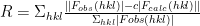
Where 


It is possible that some the atoms of different copies of the protein clash. This is not physically possible, and model placements with clashing atoms are less likely to be accurate than models without clashing atoms. Thus the following clash score is used

when 
Training
The training set consisted of 1387 protein structures. First we took 40 proteins randomly from the PDB (Protein Data Bank), a public repository of protein structures. For each of these proteins we generated protein structures of varying fidelity to the original protein structure. Some of these structures are very similar to the original structure, some are dissimilar from the original structure, and some are in between. MR-REX is run on each of the 1387 training set protein structures, and for each of them 300 candidate placements are generated. It is hoped that the model will be able to find a correct placement for each of the 1387 protein structures. For each of the models tested 40 fold cross validation was used. Repeatedly structures generated from one protein is left out and the model is trained on the structures generated from the remaining 39 proteins. The model is tested on the structures generated from the protein that was left out. The number of correct placements for the structures generated from the protein that was left out is found. This is performed for all of the proteins, one at a time, and the number of correct placements is summed. Different sets of features are tested. First each of the features is tested alone and then the most successful. Then a combination of the most successful feature and the remaining features are tested. This process was repeated until all of the features had been tested. For each of the models the raw features and the Z-scores of the features were used.
Linear Combination
The simplest thing to do is to use a linear combination of the features.

The following table shows the results of the cross validation.
| # of Features | # of Successes |
| 1 | 507 |
| 2 | 511 |
| 3 | 514 |
| 4 | 540 |
| 5 | 546 |
| 6 | 546 |
For some of the metrics the average can very greatly from protein to protein. Thus, some type of normalization seems reasonable, and I tried to use the Z-score instead of the raw features. The following table lists the results.
| # of Features | Raw Scores | Z-scores |
| 1 | 507 | 507 |
| 2 | 511 | 516 |
| 3 | 514 | 524 |
| 4 | 540 | 551 |
| 5 | 546 | 553 |
| 6 | 546 | 554 |
There was a slight improvement when using the Z-scores. The results are not statistically significant, but it is encouraging. I then ran MR-REX on a subset of 605 the protein structures using a linear combination of the raw scores and a linear combination of the Z-scores. This set of 605 proteins excluded the proteins that were too easy and almost guaranteed to succeed and the proteins that were too hard and almost guaranteed to fail. Using the raw scores there were 202 successes and when using the Z-scores there were 216 successes.
Naive Bayes
Naive Bayes is a common technique in machine learning. It is illustrated by the figure below. In the upper left we see a plot of the probability density versus R for successes (red) and failures (blue), derived from the training set. Below that is the probability of a placement being correct (successful) versus R. For example when R is 0.45, we see that we have some successes and no failures. That means that if R is 0.45 we can be 100 % sure that the placement is correct. On the other hand if R is 0.6, we see that there are no successes and some failures. That means that if R is 0.6 the probability of the placement being correct is 0. In between about R=0.5 and R=0.57 there is a region with both failures and successes. There we can obtain the probability of success by dividing the probability density of success by the sum of the probability density of success and failure. We can do the same for the other features. On the right is the corresponding plots for the clash score between core and surface atoms. To the right of that is the equation for Naive Bayes. Naive Bayes assumes that the features are not correlated.

The following table gives the results for linear combination and Naive Bayes.
| # of Features | Linear Combination | Naive Bayes |
| 1 | 507 | 485 |
| 2 | 516 | 517 |
| 3 | 524 | 544 |
| 4 | 551 | 546 |
| 5 | 553 | 541 |
| 6 | 554 | 532 |
Unfortunately Naive Bayes does worse. Naive Bayes was performed using the raw features and the Z-scores of the features. Here only the results for the Z-scores are shown as they were better than using the raw scores.
Principal Component Analysis Bayes
I had expected that Naive Bayes would outperform a linear combination of the metrics. My hypothesis for why Naive Bayes did poorly is the correlation between the different features, meant that it was not giving accurate probabilities. Principal Component Analysis (PCA) is usually used to reduce the number of features, but it also creates new features from linear combinations of the features, such that the correlation is removed. Thus, it seemed reasonable to me to remove the correlation using PCA before applying Naive Bayes. The table below shows those results with the previous results included.
| # of Features | Linear Combination | Naive Bayes | PCA |
| 1 | 507 | 485 | 518 |
| 2 | 516 | 517 | 491 |
| 3 | 524 | 544 | 485 |
| 4 | 551 | 546 | 475 |
| 5 | 553 | 541 | 470 |
| 6 | 554 | 532 | 456 |
Here all of the features are used to do the PCA, but the # of Features is the number of components used.
Split Principal Component Analysis Bayes
In the previous analysis using PCA the principal components were found using all of the data. Here PCA is performed separately for the correctly placed models and incorrectly placed models. The motivation for this is that the principal components for these two categories might be significantly different and success and failures could be better separated if PCA is done separately on them. Unfortunately the results still were not better than a linear combination of features. I think the reason this method does not work well is that the meaningful data is in the first component.
| # of Features | Linear Combination | Naive Bayes | PCA | Split PCA |
| 1 | 507 | 485 | 518 | 526 |
| 2 | 516 | 517 | 491 | 516 |
| 3 | 524 | 544 | 485 | 454 |
| 4 | 551 | 546 | 475 | 429 |
| 5 | 553 | 541 | 470 | 495 |
| 6 | 554 | 532 | 456 | 504 |
Sum of Gaussians
The thinking with the Bayesian methods was to model the distribution of failures and successes in the feature space and use that to calculate the probability that a given set of features corresponds to a failure or a success. One way to model the distribution of successes and failures is to convolute the data with Gaussians. The following equations demonstrate what I mean

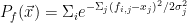
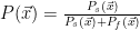
where 

Here are the results.
| # of Features | Linear Combination | NB | PCA | Split PCA | Gaussians |
| 1 | 507 | 485 | 518 | 526 | 517 |
| 2 | 516 | 517 | 491 | 516 | 533 |
| 3 | 524 | 544 | 485 | 454 | 528 |
| 4 | 551 | 546 | 475 | 429 | 522 |
| 5 | 553 | 541 | 470 | 495 | 519 |
| 6 | 554 | 532 | 456 | 504 | 497 |
The sum of Gaussians method gets off to a promising start but then goes down hill. I believe that this method requires more data to work well when working with large dimensional data than the other methods and that is why its performance gets worse. The lesson here is that sometimes the simpler methods work best.