

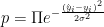
Maximum likelihood is the procedure of finding the value of some parameters for a given statistic which makes the likelihood of the the known likelihood distribution a maximum. Maximum likelihood is a method with many uses. A classic example is linear regression. If it is assumed that the errors on the x variable follow a Gaussian distribution we can compute the probability density of the parameters used to fit the data. A Gaussian distribution is given by

where 

If we draw a line and ask what is the probability density that we see the observed data given that if we had an infinite amount of data and the mean of the Gaussian distributions for each y value is centered on a line, then we obtain the equation

where 
It is more convenient to take the natural log of both sides, since that converts the product into a sum and does not change the location of the maximum. In that case we obtain

Again we do not care about any constant factors so we can get rid of 

If we want to do a minimization instead of a maximization we can change the sign

This is the purpose for doing least squares regression as opposed to say least quartic regression or minimizing the sum of the absolute values of the errors. We can now find the slope and y-intercept of the model.
Maximum Likelihood Applied to X-ray Crystallography
Let’s look at a more complicated use of the maximum likelihood technique. As a postdoctoral fellow I wrote a software package MR-REX, which helps determine protein crystal structures given X-ray crystallographic data and an initial guess for the structure of the protein, using a technique known as MR (Molecular Replacement). I described it in an earlier blog post here. In order for MR-REX to work it needs a quantitative measure of how well the calculated X-ray scattering amplitudes, of a hypothetical placement of a protein model, matches the observed scattering amplitudes. For this, MR-REX used a liner combination of terms, one of which is likelihood. I did not invent the use of maximum likelihood for X-ray crystallography, but I did spend a lot of time trying to understand it and deriving it by myself. You can find some interesting information about the use of maximum likelihood in X-ray crystallography here. If the maximum likelihood score was a true maximum likelihood score, it should be the only term used to assess how well the calculated and observed match, but there are some approximations used in its derivation in this case. In a test set of 320 runs of MR-REX, the maximum likelihood score alone picked out the correct placement of the protein model in 123 cases compared to 114 for the R factor. We start off with the equation for the intensity of the scattered X-ray light.
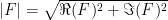
where F is the structure factor, j specifies the index of the atom, h, k, and l are the Miller indices, x, y, and z specify the coordinates of the atoms, f is the structure factor of the atom, O is the occupancy of the atoms, and B accounts for the thermal motions of the atoms. The intensity is calculated by multiplying the structure factor by its complex conjugate and the amplitude is the square root of the intensity. The structure factor is a complex number with real and imaginary components. Only the intensity of the scattered X-ray light can be measured. The real and imaginary components of the structure factor cannot be measured. If we assume that there is some error in the positions of the atoms with a Gaussian distribution, there will be an error in the real and imaginary components of the structure factors with a Gaussian distribution. The errors on the real and imaginary components are either completely uncorrelated (acentric reflection) or the real and imaginary components lie on a straight line when plotted (centric reflection). Centric reflections result from symmetry relations between different copies of the protein in the unit cell. Centric reflections are easier to analyze so let’s start with them.
Likelihood for Centric Reflections
Let’s say that the real component of a centric reflection is $latex{Fave}$ and the standard deviation of the real component of a centric reflection is 

The probability density that the structure factor is -F is then given by

Since


This is known as the Woolfson distribution.
 is 1.0. The amplitude |F| is always positive, so P(|F|) is obtained by flipping over P(F) for negative values of F and adding that to P(F) for positive values of F.
  is 0.3.
 The overall likelihood of all of the centric reflections is

This involves multiplying thousands of very small numbers together, resulting in floating point underflow. Thus, we take the log of both sides.

Acentric Reflections
Let’s next look at acentric reflections. Let’s say that the expected real component of the structure factor is Fave, that its standard deviation is

In the case under consideration

where 


To find 


WolframAlpha tells me that the result is

where 
 is 1.0 and on the right is 0.3.
 We can then find the overall log likelihood for the acentric reflections

The overall log likelihood is then

Calculating

We assume that there is some error with the x, y, and z coordinates of the atoms with standard deviations 


where the atom is located at (x, y, z) in the model. The standard deviations themselves are estimates, which is typically based on the sequence identity of the model. The higher the sequence identity the smaller the estimated standard deviations.
Let’s return to the equation for the structure factor

Let’s rewrite this for just one atom

We need to look at the standard deviations of the real and imaginary components of the structure factor, so we need to look at the real and imaginary components of the structure factor.


The standard deviation, 

We can find the average real component of the structure factor using

Similarly

Variances are additive, assuming that the errors on the positions of the atoms are uncorrelated. Therefore we can find the total variance by summing up the variances due to each individual atom.

I leave it up to the interested reader to find the full equation for 